Monday, September 22, 2014

air sensors coming along

I've got a team focusing on air sensors.  So far, we've focused on the MQ series.  You get what you pay for, so these are the most reliable devices.  They operate with a heated element to produce a redox voltage, much like an oxygen sensor in your car does.


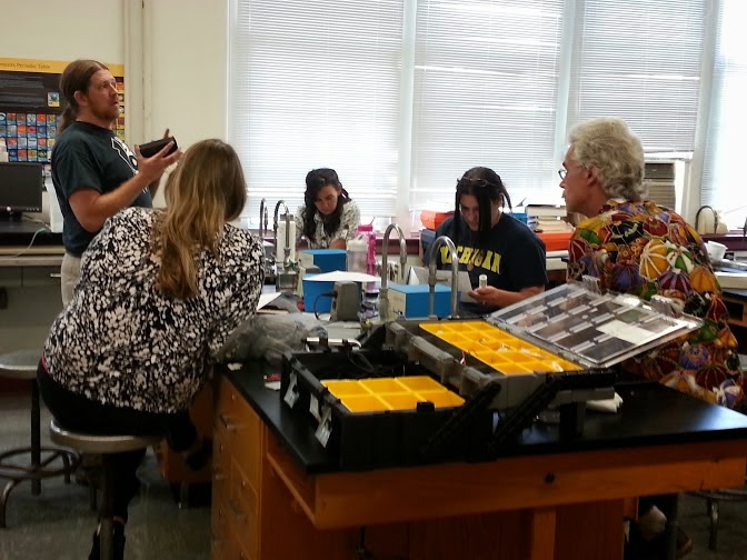
Pictured above is a very amateurish attempt at calibrating an MQ-2 methane sensor.  The natural gas in the chemistry lab, like most commercial gas, is about 96 percent pure, so in theory, a saturation of it would be 960,000 ppm.  Don't laugh, I know that's not what's happening here.  We're trying to teach theory, not reality, on this one.  We pumped a line from a gas valve into this cloche and looked for a max value on the analog to digital read.  In this case, it maxed at about 970.  The low that we get for this sensor is 54.   The data sheet for the mq sensors has them calibrated on a logarithmic scale.  We got our constant this way:

960000=10k(970-54)  or     max val ppm= 10 k (max analog read-min analogread)
Log 960000 =  k(916)
Log960000/916 = k = .006530864

so the final formula that converts the analog read to ppm is based on the formula:

Y= 10 ^ .006530864(x-54)                         x being the analog read value


The math in the Arduino sketch would go this way:

void loop() {

  // read the analog in value:
  // read the sensor:
  int sensorReading = analogRead(A0);
    float ppmValue = pow(10,(.006530864*(sensorReading-54)));
  // print the sensor reading so you know its range
    Serial.print("ppm methane = " );                      
  Serial.println(ppmValue);


We can think of half a dozen reasons off the top of our heads to not trust whatever number is spewing out, but in theory, it gets the principle of calibrating and constants taught.  If we're lucky, we might track down some really accurate monitoring devices for our pollutants  that we can calibrate against to get our own readings somewhere in the ballpark.  

Friday, September 12, 2014

Finally out in the field

We went out in the field with Dr. Mark Schorr from the University of Tennessee at Chattanooga.  Dr. Schorr has been sampling the North Chickamauga system for decades, and looks forward to getting data from our project.

We first went to an acid mine damage mitigation site, which has a four stage containment pond system:  plastic lining and limestone:

You can see the "yellowboy", better known as precipitated/oxidized iron.  Good time for a bit of brushup on pH, negative logs, and redox.
 We had the xbee radios attached to our equipment available if needed to save time getting around to different sampling points.  Didn't really need them, though it was nice to have them out...

At our reference stream, we did some old-style colorimetric titrations for parameters like alkalinity and hardness.


After leaving the mitigation site, we went to our reference/baseline stream. 
I threw some botany and geology while we were out there, which I always try to do on a field trip.  The kids had a great time, and as one student remarked, "Now all this seems more real.  I have a more thorough understanding of what we're trying to accomplish."


Got the first skyping in

Goal is every Thursday to have a tutorial and conference.  Since my kids will be in other classes when the Hixson kids are available, we'll just rotate a pair of team ambassadors each time.

Prepping for the First Field Trip

Our team met early this week.  Dr. Schorr from UTC was with us.  We got down to the brass tacks of the field trip, but also the design challenges of getting buoys out in the streams that will work long term.  Looking forward to seeing the prototypes that the kids at Hixson are coming up with.


Wednesday, September 3, 2014